| AP Statistics |
|
|
|
| Sections: 1.| Inference for a Population Proportion 2.| Comparing Two Proportions |
|
|
|
Comparing Two Proportions There's really nothing new to learn to compare two proportions because we know how to compare means. Proportions are just means! The proportion having a particular characteristic is the number of individuals with the characteristic divided by total number of individuals. Suppose we create a variable that equals 1 if the subject has the characteristic and 0 if not. The proportion of individuals with the characteristic is the mean of this variable because the sum of these 0s and 1s is the number of individuals with the characteristic. The Sampling Distribution of
Both
Using these facts gives us some important information about
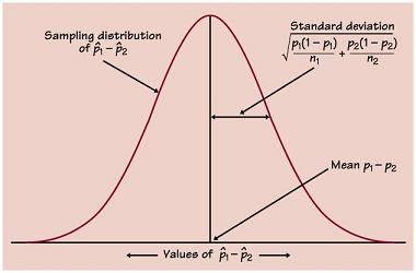
the sampling distribution of
The figure below illustrates the distribution of
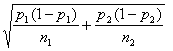
Confidence Intervals The standard deviation of
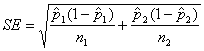
To obtain a confidence interval replace the population
proportions p1 and p2 in the expression by the sample
proportions. the result is the standard error of the statistic
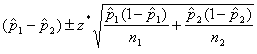
The formula for the confidence interval has the form estimate ± z*SEestimate
Even though this looks different from other formulas we've seen, it's nearly identical to the formula for the "equal variances not assumed" version of Student's t test for independent samples. The only difference is that the standard deviations are calculated with n in the denominator instead of n-1. Example: Suppose that in a sample of 68 urban students, 42 have had a flu shot and in a sample of 65 rural students, 30 have had a flu shot. The two sample proportions are 0.800 and 0.462. Data summary: n1 = 68,
Check assumptions: the smallest value of
A 95% confidence interval for the difference in population proportions is
= 0.156 ± 0.167 = (-0.011, .323) We can be 95% confident that the proportion of urban students with flu shots is between -1.1% and 32.3 different than the proportion of rural students with flu shots. This confidence interval is fairly wide because the sample sizes are small. Try Self Check 18 Significance Tests We want to investigate the differences between two sample proportions from two distinct populations. Is there a true difference in the proportions or is the difference due to chance. To test the null hypothesis H0: p1 = p2 against a one- or two-sided alternative hypothesis Ha, first compute a pooled estimate for the parameter, where X1 and X2 represent the number of "successes" in each population sample. This estimate for a single sample proportion agrees with the null hypothesis, where the two proportions are assumed to be equal. Calculate the pooled standard error SE, which is equal to 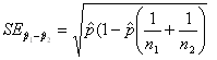 The test statistic z =
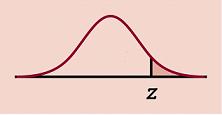
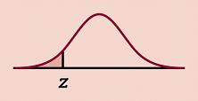
P(Z > z) for Ha: p1 >
p2 Example: Students in grades 4-6 were asked whether good grades, athletic ability, or popularity was most important to them. Is popularity more important to girls or boys? 169 girls and 166 boys were included in the survey. Of the girls, 58 ranked popularity most important, compared to 40 of the boys. The sample proportion
Null hypothesis H0: p1 = p2 Alternative hypothesis Ha: p1 ≠ p2 To test the difference of the proportions of girls and boys who rated popularity most important, first compute the pooled estimate
Using this value we need to check our conditions to see if a 2-sample z procedure is valid.
All are clearly greater than 5 so we are safe to use the two-sample z procedure. Calculate the standard error using
SE = 0.0497 The test statistic is
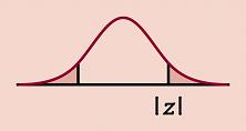
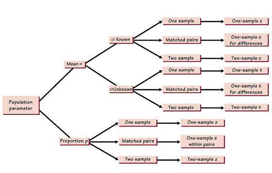
Since this is a two-sided hypothesis, we are interested in the probability 2P(Z > 2.05) = 2(1 - P(Z < 2.05)) = 2(1 - 0.9798) = 2(0.0202) = 0.0404. Conclusion: Since the p-value is small it may be safe to say that girls in grades 4-6 find popularity to be more important than boys in grades 4-6. Notice that the finding is significant at the 0.05 level, although it is not significant at the 0.01 level. Try Self Check 19 Below is a flow chart that will help you choose the correct procedures when doing inferences on means and proportions. You are not allowed to use this chart on the AP Statistics exam but studying it will help understand which procedure to use.
Proceed to Statistics Assignment 11: Working with Two Proportions
Proceed to the Unit 5 Exam Objective Questions and Free Response (The
Objective Questions contain 8 Multiple Choice and 8 True/False.) |
|
© 2004 Aventa Learning. All rights reserved. |