| AP Statistics |
|
|
|
| Sections: 1.| Density Curves 2.| Normal Distributions 3.| Normal Distribution Calculations 4| Assessing Normality |
|
|
|
Normal Distributions The normal curve is called a family of distributions. Each member of the family is determined by setting the parameters ( μ and σ ) of the model to a particular value (number). Because the μ parameter can take on any value, positive or negative, and the σ parameter can take on any positive value, the family of normal curves is quite large, consisting of an infinite number of members. This makes the normal curve a general-purpose model, able to describe a large number of naturally occurring phenomena, from test scores to the size of the stars.Similarity of Members of the Family of Normal CurvesAll the members of the family of normal curves, although different, have a number of properties in common. These properties include: shape, symmetry, tails approaching but never touching the x-axis, and area of 1 under the curve.
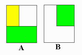
All normal distributions have the same overall shape. The exact density curve for a particular normal distribution is described by giving its mean μ and its standard deviation σ. The mean is located at the center of the symmetric curve, and is the same as the median. Changing μ without changing σ moves the normal curve along the horizontal axis without changing its spread. The standard deviation controls the spread of a normal curve.Area under a curve Because area under a curve may seem like a strange concept to many introductory statistics students, a short intermission is proposed at this point to introduce the concept. Area is a familiar concept. For example, the area of a square is s2, or side squared; the area of a rectangle is length times height; the area of a right triangle is one-half base times height; and the area of a circle is π * r2. It is valuable to know these formulas if one is purchasing such things as carpeting, shingles, etc. Areas may be added or subtracted from one another to find some resultant area. For example, suppose one had an L-shaped room and wished to purchase new carpet. One could find the area by taking the total area of the larger rectangle and subtracting the area of the rectangle that was not needed, or one could divide the area into two rectangles, find the area of each, and add the areas together. Both procedures are illustrated below:
Finding the area under a curve poses a slightly different problem. In some cases there are formulas which directly give the area between any two points; finding these formulas are what integral calculus is all about. In other cases the areas must be approximated. Suppose a curve was divided into equally spaced intervals on the x-axis and a rectangle drawn corresponding to the height of the curve at any of the intervals. The rectangles may be drawn either smaller that the curve, or larger, as in the two illustrations below:
In either case, if the areas of all the rectangles under the curve were added together, the sum of the areas would be an approximation of the total area under the curve. In the case of the smaller rectangles, the area would be too small; in the case of the latter, they would be too big. Taking the average would give a better approximation, but mathematical methods provide a better way. A better approximation may be achieved by making the intervals on the x-axis smaller. Such an approximations is illustrated below, more closely approximating the actual area under the curve.
The actual area of the curve may be calculated by making the intervals infinitely small (no distance between the intervals) and then computing the area. If this last statement seems a bit bewildering, you share the bewilderment with millions of introductory calculus students. At this point the introductory statistics student must say "I believe" and trust the mathematician or enroll in an introductory calculus course.
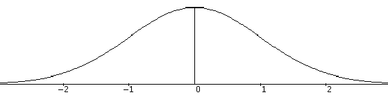
Looking at the normal curve
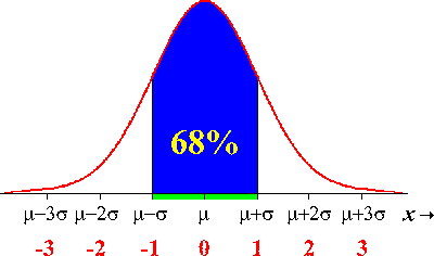
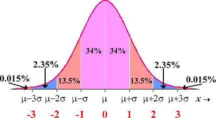
The normal curve above shows relative positions of the standard deviation. Notice how the curve "turns" at the points -1 and 1. The points at which this change of curvature takes place are called inflection points and are located at distance σ on either side of the mean μ. Remember that μ and σ alone do not specify the shape of most distributions, and that the shape of density curves in general does not reveal σ. These are special properties of normal distributions. The σ controls the shape of the normal curve. If σ is large the normal curve will extend far down the x-axis and the graph will be "flat". A small σ will increase the height of the graph as well as narrowing the spread.Why are the normal distributions important in statistics? Here are three reasons. First, normal distributions are good descriptions for some distributions of real data. Distributions that are often close to normal include scores on tests taken by many people (such as SAT exams and many psychological tests), repeated careful measurements of the same quantity, and characteristics of biological populations (such as lengths of cockroaches and yields of corn). Second, normal distributions are good approximations to the results of many kinds of chance outcomes, such as tossing a coin many times. Third, and most important, we will see that many statistical inference procedures based on normal distributions work well for other roughly symmetric distributions. However, even though many sets of data follow a normal distribution, many do not. Most income distributions, for example, are skewed to the right and so are not normal. Nonnormal data, like nonnormal people, not only are common but are sometimes more interesting than their normal counterparts.The 68–95–99.7 rule Although there are many normal curves, they all have common properties. In particular, all normal distributions obey the following rules. Approximately 68% of the observations fall within 1 standard deviation of the mean |
|
© 2004 Aventa Learning. All rights reserved. |


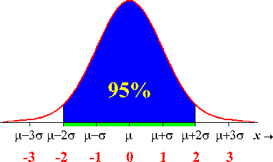
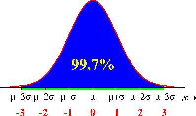
 Connection: If 99.7% of the data is "contained" within 3 standard deviations
of the mean, plus and minus, then the standard deviation could be estimated
by the range. If we know the range of a distribution that is approximately
normal then it would be safe to estimate the standard deviation by
(range/6). Also you can use the standard deviation to estimate the range, 6σ
would be a good estimate of the range.
Connection: If 99.7% of the data is "contained" within 3 standard deviations
of the mean, plus and minus, then the standard deviation could be estimated
by the range. If we know the range of a distribution that is approximately
normal then it would be safe to estimate the standard deviation by
(range/6). Also you can use the standard deviation to estimate the range, 6σ
would be a good estimate of the range.