Learn
Graphing Linear Equations
What is a linear equation
A linear equation involves one or two variables, typically denoted as x and y. In a linear equation, these variables are only raised to the first power, which means you won't find variables in the denominator of a fraction, inside a radical, or raised to any power greater than 1.
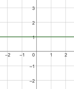
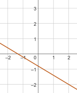
These are some equations and graphs of linear equations. Their graphs form straight lines:
y = 1
−3x − 5y =4
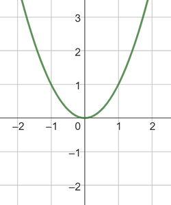
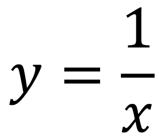
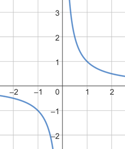
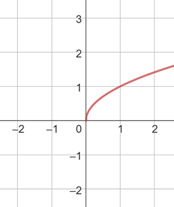
Now compare those linear graphs to the equations and graphs of non-linear equations. Their graphs form curves:
y=x²
![]()
Recall that the y is called the dependent variable. We call this set the range.
The x is called the independent variable becuase the value of y is dependent upon the value of x. We call this set the domain.
We will continue reviewing graphing linear equations. You can graph linear equations using the slope-intercept form that you reviewed in the previous lesson, or you can graph linear equations by finding the x and y-intercepts.
Example #1
Watch Graph Linear Equations Using X and Y Intercepts and One More Point.
Open Graph Linear Equations Using X and Y Intercepts and One More Point in a new tab
Note: The presentation may take a moment to load.
Graphing Linear Equations
Graphing Inequalities
Remember when graphing inequalities on a number line, we marked an open or closed endpoint then drew a line in one direction. Graphing linear inequalities is done in a similar manner.
To graph y ≤ x -2, we first draw a boundary line which is the graph of the equation y = x -2. The boundary line will be solid for inequalities with ≥ or ≤. The boundary line will be a dashed line for inequalities with < or >.
Next, we will shade to one side of the line. To decide which way to shade, we choose any point that is not on the boundary line and substitute it into the inequality. If the point makes the inequality a true statement, then the point is a solution, so we shade the side of the graph that contains the point we tested. If it is a false statement then the point is not a solution, so we shade the other side.
Example #2
Watch Graph Linear Inequalities Using a Table of Values.
Open Graph Linear Inequalities Using a Table of Values in a new tab
Note: The presentation may take a moment to load.
Example #3
Watch Graph Linear Inequalities Using a Table of Values.
Open Graph Linear Inequalities Using a Table of Values in a new tab
Note: The presentation may take a moment to load.
More Linear Inequalities
Linear Inequalities
Another way to graph linear inequalities is to write in slope-intercept form, find and plot the y-intercept, and then apply the slope (rise over run) to find the next point.
Example #4
Watch Graph Linear Inequalities Using Slope and Y-Intercept.
Open Graph Linear Inequalites Using Slope and Y-Intercept in a new tab
Note: The presentation may take a moment to load.
Example #5
Watch Graph Linear Inequalities Using Slope and Y-Intercept.
Open Graph Linear Inequalites Using Slope and Y-Intercept in a new tab
Note: The presentation may take a moment to load.